September 2026
On the 19th of August I had five free hours and a message in the guild chat about an AI contest in December. I figured the quickest way to find out what I didn't know was to enter a Kaggle competition that same afternoon. I also wanted something to post on LinkedIn. I'm not going to pretend otherwise.
I had never entered one before. Twelve days later I finished 351st of 3,532 teams on one leaderboard and 369th on the other, which is the top ten percent on one and a hair outside it on the other. This is the whole thing in order, written for the version of me who opened the page on day one and didn't know what any of the words meant.
What a Kaggle competition actually is
You get two files. train.csv has 691,369 rows, each one a person, with twelve columns about them (hours of screen time, hours on social media, hours gaming, hours of sleep, notifications per day, age, and so on) plus one final column called addicted_labelthat's 1 or 0. That last column is the answer.
The first three rows look like this, one column per person.
| column | person 0 | person 1 | person 2 |
|---|---|---|---|
| id | 0 | 1 | 2 |
| age | 24.0 | 19.0 | 18.0 |
| daily_screen_time_hours | empty | 5.97 | 5.09 |
| social_media_hours | 1.83 | 1.08 | empty |
| gaming_hours | 1.59 | empty | empty |
| work_study_hours | 2.11 | 3.03 | empty |
| sleep_hours | 7.46 | 8.22 | 6.25 |
| notifications_per_day | 122.0 | 76.0 | 134.0 |
| app_opens_per_day | 38.0 | 19.0 | 60.0 |
| weekend_screen_time | 8.63 | empty | 7.47 |
| gender | Male | Female | Female |
| stress_level | Medium | Medium | Low |
| academic_work_impact | No | No | Yes |
| addicted_label | 1 | 0 | 0 |
The gaps are real. Person 0 has no screen time recorded, person 2 is missing three of the hour columns, and only 595,515 of the 691,369 rows carry all four of the hour columns at once. That matters later, because the strongest thing I found in this data only exists in the rows that have all four.
test.csv has 296,000 more people and no answer column. Your job is to guess. You upload a two-column file, one row per person, in this shape.
id,addicted_label
691369,0.8421
691370,0.1337
691371,0.9002
That second number is a confidence between 0 and 1 rather than a yes or no, which I hadn't expected. Kaggle scores the file, puts you on a leaderboard, and lets you upload five times a day. The competition I entered was Playground Series Season 6, Episode 8, which ran from the start of August to the 31st. Playground competitions are the practice tier, with no prize money, thousands of entrants, and the data is generated rather than collected, which matters later.
The score, and why it isn't accuracy
The metric here is ROC AUC. It took me a few tries to get it, and this is the phrasing that stuck.
Take one person who really is addicted and one who really isn't, both at random. Look at the two numbers your model gave them. Did it give the addicted one the higher number? AUC is simply how often that's true. Guess randomly and you're right half the time, so 0.5. Get it right every time and you score 1.0.
The important part is that AUC only cares about the order, not the actual values. A model that outputs 0.9 and 0.8 scores the same as one that outputs 0.02 and 0.01, as long as the right person is on top. This is why you submit probabilities and never round them to 0 and 1. Rounding throws away the ordering inside each group and your score collapses. I know because the first thing I wanted to do was round them.
The first hour
The baseline was LightGBM, a gradient boosting library, run five times over the data with default settings. It took about ten minutes to write and run. It scored 0.96487 on the leaderboard. The person in first place had 0.97134.
My first question was how anyone finds the extra 0.0065, and my second was whether 0.0065 is even a lot. On this problem it is, because the entire field lives inside about half a percent. A ten-minute script put me within 0.65 percent of first place, and the remaining twelve days went on the last 0.006. I had assumed the gap between a beginner and the top would be wide, and most of it closed in ten minutes.
The second thing I tried was adding a second library, XGBoost, and averaging the two sets of guesses. The score moved by 0.0004. I asked what that had actually done and why it worked, which turned out to be the question I kept asking for the rest of the week.
Cross-validation, and why the leaderboard lies
I didn't know what a fold was. A fold is one of the equal chunks the training data gets cut into. With five folds you train on four of them, predict the fifth, rotate until every chunk has been predicted once by a model that never saw it, then average the five scores. That average is called your CV, and it is your own private leaderboard.
It matters more than the public one. The public leaderboard is scored on a slice of the test set, and every time you look at it and change something in response, you're quietly fitting your model to that slice. Do it fifty times and your leaderboard score is measuring how well you memorised the leaderboard.
The one genuinely useful thing to do with the public score is to check it once against your CV at the start. Mine agreed to within 0.002, with the leaderboard slightly higher than CV. Had it come in below CV I would have known my folds were flattering me. From then on I only submitted when CV went up, and I put the CV number in every submission description so I could tell later what had actually helped.
Leakage
Leakage is when your model sees something during training that it won't have at prediction time. The textbook example is a model that predicts whether a patient has diabetes from a set of columns that includes "is taking insulin". The model scores 0.99 and is useless, because in real life the insulin comes after the diagnosis you're trying to predict.
The cheap check is to score every column on its own against the answer. If one column nearly solves the problem by itself, something is wrong. Here the strongest were daily screen time and weekend screen time, and neither came close to solving it alone.
The subtler version bit other people. Target encoding is a common trick where you replace a category with the average answer for that category. Do that beforeyou split into folds and each fold's training data now contains a summary of its own validation answers. Several popular public notebooks did exactly this. Their validation scores were beautiful and their leaderboard scores weren't. Until then I had thought of leakage as a mistake careless people make. It's also a mistake careful people make when the loop is one line too short.
What the data generator left behind
Playground data is synthetic. Kaggle takes a real dataset, trains a model to imitate it, and generates hundreds of thousands of fake rows. This one came from a 7,500-row survey that the competition page credits. The imitation is never perfect, and the imperfections are where most of the gain over the baseline came from.
The first one you can see by counting. Screen time is recorded to two decimal places, so across 691,369 people you would expect almost no exact repeats. Instead there are only 1,389 distinct values in the whole column, and the most common one shows up 3,434 times.
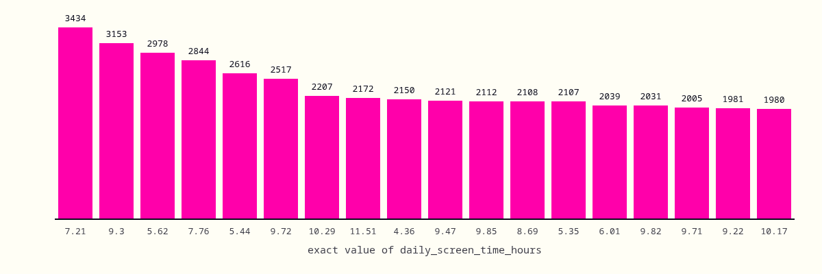
Once you see that, the column stops being a measurement and starts being a set of labels that happen to look like numbers. Converting them to text and treating them as categories moved my score more than any hyperparameter did.
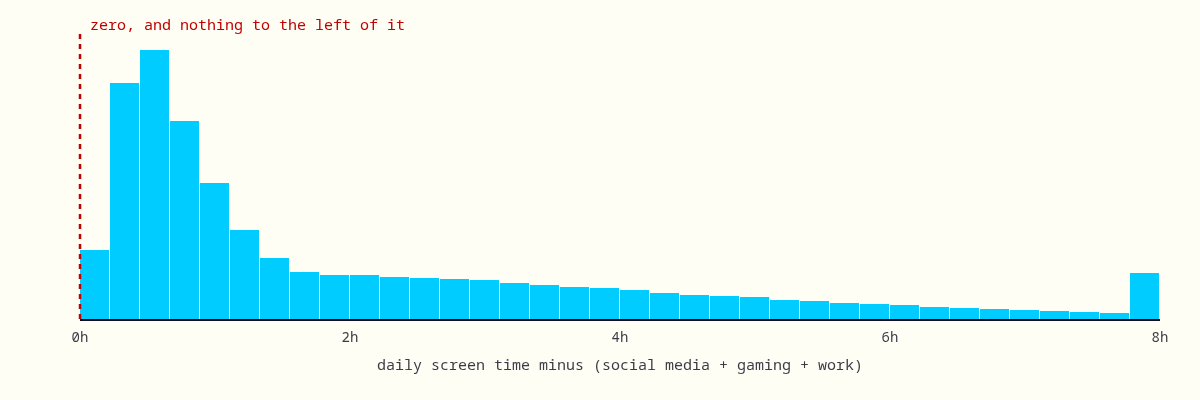
The second one is a rule. In the generated data, daily screen time is never less than social media plus gaming plus work hours. That holds in all 595,515 rows that have all four values, without a single exception. The real survey breaks that rule in more than half its rows, so the generator was enforcing something the humans didn't. The size of the gap, which I started calling slack, predicts the answer at 0.765 AUC entirely on its own.
I also tried the obvious cheat. If the fake data came from a real survey, why not just find the survey and use the real answers? I found it, confirmed it was the source, and added it to the training data. The score got worse, from 0.96632 to 0.96628 with one copy, and to 0.96596 with ten. The generator had re-invented the answers from scratch, so the real ones had nothing to say about the fake people.
Eighty-four models
The last stretch was volume. By the end there were 84 different models. LightGBM, XGBoost and CatBoost across different random seeds and fold counts, plus a small neural network that treats each column as a word in a sentence, which I took from a public notebook after my own attempt at one came out worse.
You then have to combine 84 sets of guesses into one. I tried three ways of doing it and they all landed within 0.0001 of each other, which told me the combining method wasn't where the score lived. What did move it was adding a model that made different mistakes from the others. Another copy of the same model with a new random seed was worth about 0.00003.
Forking the public notebook
Partway through I noticed a lot of identical scores on the leaderboard. That happens when one public notebook, itself a blend of other public notebooks, gets forked by everyone who opens it. Kaggle breaks exact ties by who submitted first, so a chunk of the board was ordered by submission time rather than by anything the models did.
On August 23 I joined it, submitting the blend verbatim with the description "public blend, forked, max public". It scored 0.97117 and put me at rank 98 of 2,687. I took a screenshot. I want to be clear that the number wasn't mine.
By the deadline the same file was rank 351 of 3,532. Nothing about it had changed. The notebook kept being improved and re-forked, and the newer forks piled into clusters above mine, 72 teams tied at 0.97128 and 71 at 0.97130, with 344 teams above me in total. My file sat still while the people around me kept improving theirs.
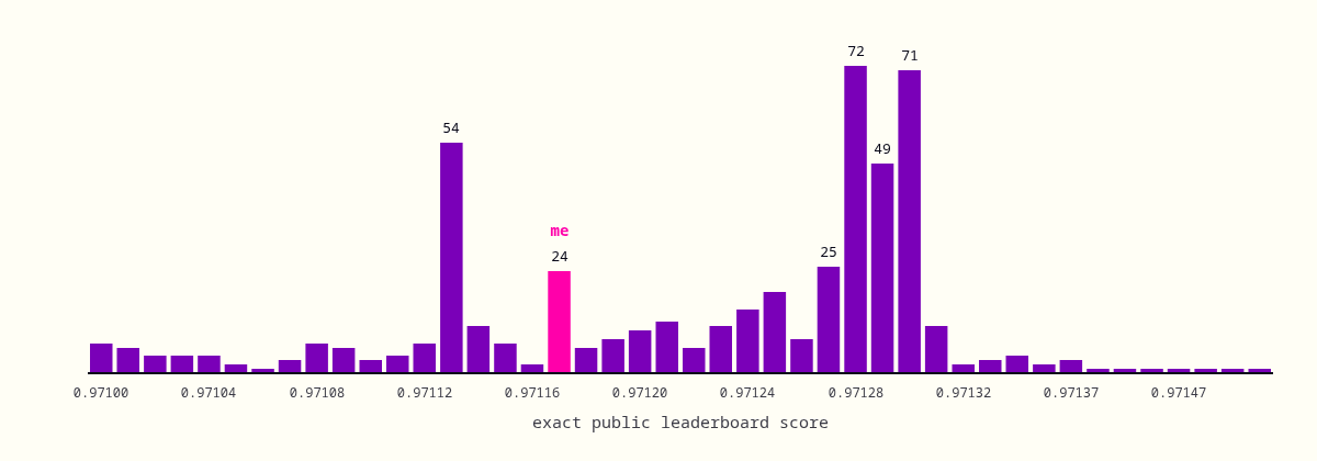
The fork handed me a score that other people were already busy improving on. I don't think I'd have understood that from reading about it.
The two finals
Kaggle scores you twice. The leaderboard you watch all competition is computed on a slice of the test set. The real one, scored on everything else, is hidden until the deadline. You pick two submissions to be judged on it.
One of my slots went to the fork. The other went to the best thing I had built myself, a fifteen-seed bagged ElasticNet stack, CV 0.96998, public 0.97101. My theory was that the fork was fitted to the public slice and would fall, the honest entry would hold, and I'd come out ahead of the queue.
On September 1 the fork went from 0.97117 to 0.97090, and the honest entry from 0.97101 to 0.97071. Both dropped by about the same amount, the fork still won, and I landed at 369th. The theory was wrong, or the effect was too small to see. The winner, Chris Deotte, scored 0.97207 public and 0.97176 private, clear of every cluster on both boards.
His writeup is not what I expected. He ran a swarm of language model agents, set two of them competing to build the best single model, and one of those models won the competition on its own, without an ensemble, which he says had not happened in a Playground competition in eighteen months. The comments underneath are worth reading too, because a lot of people finishing a few hundred places above and below me were asking the same question about what is left for a person to do.
Second place is the one I keep rereading. Xin Feng did it by hand on Kaggle's free GPUs and a twenty dollar subscription, and his writeup lands on the same rule this post keeps circling. Trust your own out-of-fold score and treat the public leaderboard as a check rather than a target. He also says he spent his last week hunting for a better way to blend when he should have been improving one model. I made that mistake in miniature with my 84.
The thing I could not have outsourced was knowing whether to believe my own validation. Deotte says something close to this in the comments, where he writes that humans cannot beat agents on coding speed any more, only on the insight the agent overlooked. Learning what a fold is for turns out to be the part that keeps mattering.
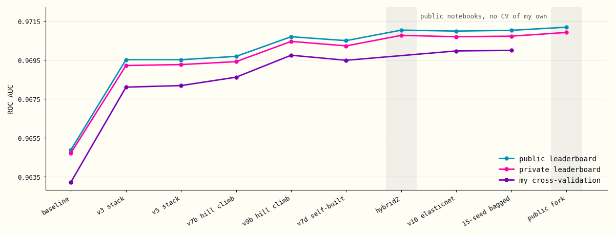
Every submission I made is public on my Kaggle profile. The table below has my own cross-validation score next to the public and private scores for each one.
| Date | Submission | CV | Public | Private |
|---|---|---|---|---|
| Aug 19 | LightGBM baseline, 5-fold | 0.96321 | 0.96487 | 0.96471 |
| Aug 19 | v3, nested target encoding, slack feature, 3-model stack | 0.96809 | 0.96950 | 0.96920 |
| Aug 19 | v5, 4-model logistic-rank stack | 0.96817 | 0.96950 | 0.96925 |
| Aug 20 | v7b, hill climb over 10 members | 0.96860 | 0.96967 | 0.96940 |
| Aug 20 | v9b, hill climb over 81 public and own OOF arrays | 0.96973 | 0.97068 | 0.97044 |
| Aug 20 | v7d, self-built final, 3 transformer seeds and 2 CatBoosts | 0.96947 | 0.97048 | 0.97021 |
| Aug 20 | hybrid2, 0.4 self-built, 0.6 public blend | 0.97102 | 0.97075 | |
| Aug 23 | v10, ElasticNet stack over 84 members | 0.96995 | 0.97097 | 0.97068 |
| Aug 23 | overnight, 15-seed bagged ElasticNet | 0.96998 | 0.97101 | 0.97071 |
| Aug 23 | the public blend, forked verbatim | 0.97117 | 0.97090 |
Ten of my fifteen submissions. The other five were the same ideas with different random seeds.
The ceiling
Somewhere around day three I asked why I couldn't simply keep going until the score hit 1.0. There is a limit built into the data itself, and it has a name.
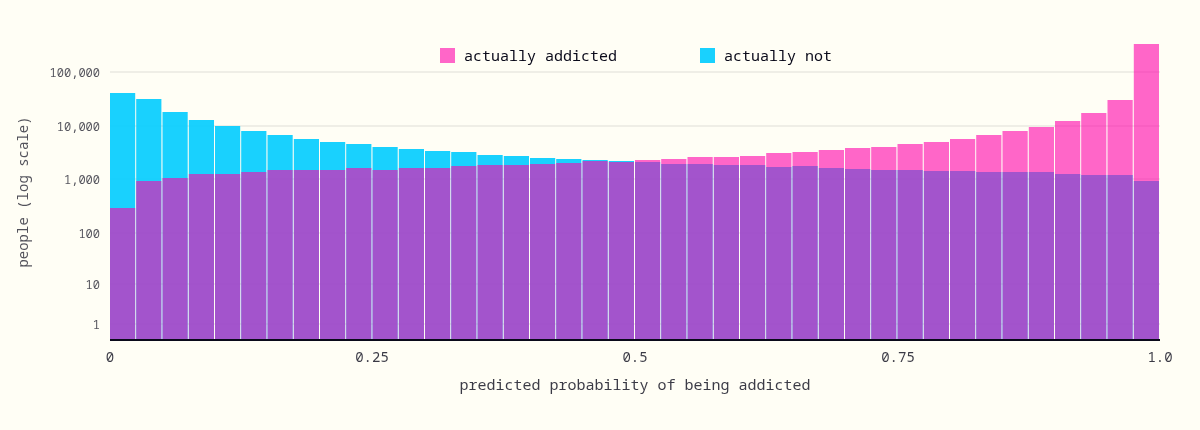
For any set of features there's a true probability that a person with those exact numbers is addicted. Call it p. If p is only ever 0 or 1, meaning the numbers fully determine the answer, then a perfect model scores 1.0. But if two people can share every number and get different answers, no model can rank one above the other, and every pair like that costs you score. The loss you can't avoid is called the Bayes error, and the best score anyone could possibly reach is the Bayes-optimal one.
You can see it in this data. Round four of the columns and group the people who match. Most of them end up in a group where the answer isn't unanimous.
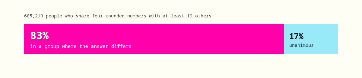
That changes what the competition was about. Everyone above 0.97 was already pressed against that ceiling, and the fight was over the last thousandth. Kaggle gives you thirty free GPU hours a week, and I spent an evening getting my own laptop's graphics card working after finding it walled off by a virtual machine config I had set up a year earlier and forgotten. None of it changed the number, because the ceiling is a property of the data and not of how fast you can train.
Whether to do it again
Halfway through I asked whether someone who doesn't especially want an AI engineering job should grind this. My answer now is that one competition teaches you what cross-validation is for, what leakage looks like when it's subtle, how to read someone else's notebook and check its claims against the raw data, and how little the last three decimals are worth. The second competition teaches you the same things again.
So I'm not entering Episode 9. The December contest is a different shape, seven hours, a team of three, no leaderboard to probe, and what carries over is the discipline rather than the models. One fixed fold split, and a submission only when the honest number moves.
What I posted on LinkedIn was the rank. What I saved was the list of questions I asked between the 19th and the 31st, starting with "why AUC" and ending with "is there a theoretical maximum a perfect model can't reach". If I had to keep one of the two, it would be the list.
Sources and further reading. The competition: Predicting Smartphone Addiction and its final leaderboard, which is where the rank and cluster counts come from, plus the winning writeup, the second place writeup and my own profile. The source survey: Smartphone Addiction Prediction Data. The libraries: LightGBM, XGBoost, and CatBoost. On the metric, scikit-learn on ROC AUC and the Wikipedia article. On the ceiling, Bayes error rate. The charts of repeated values, the slack rule and the ceiling were computed from the competition's own train.csv; the leaderboard chart from Kaggle's public leaderboard export.